PG-SUI Tutorial
Overview
PG-SUI (Population Genomic Supervised & Unsupervised Imputation) performs missing-data imputation on SNP genotype matrices using Deterministic, Supervised, and Unsupervised model families. It integrates tightly with SNPio for reading, filtering, and writing genotype datasets, and emphasizes unsupervised deep learning approaches tuned for class imbalance and diploid (3-class) genotype representations. Unsupervised neural approaches (e.g., autoencoding families) are inspired by prior work on representation learning and generative modeling (Hinton & Salakhutdinov, 2006; Kingma & Welling, 2013).
PG-SUI supports both a command-line interface (CLI) for scripted workflows and a Python API for programmatic control.
Unsupervised Models
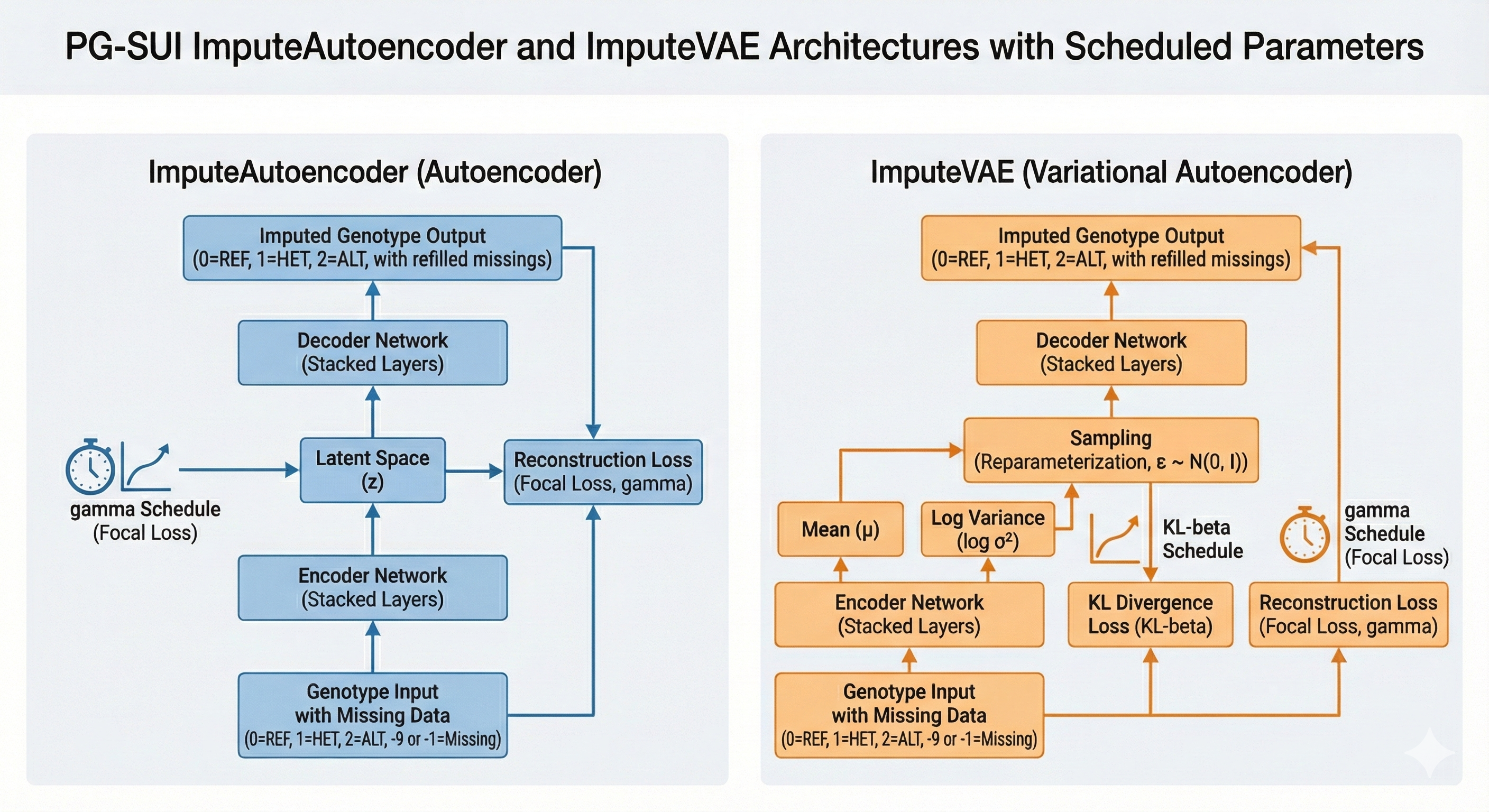
ImputeAutoencoder: Standard autoencoder architecture for genotype reconstruction (Hinton & Salakhutdinov, 2006).
ImputeVAE: Variational Autoencoder with KL regularization (Kingma & Welling, 2013).
ImputeNLPCA: Decoder-only non-linear PCA with per-sample latent embeddings and projection-based refinement.
ImputeUBP: Unsupervised Backpropagation with phased training and latent projection (Gashler et al., 2014).
These models learn structure from observed entries and then infer true missing genotypes by training on simulated missingness.
Supervised Models
ImputeRandomForest: IterativeImputer + RandomForestClassifier.
ImputeHistGradientBoosting: IterativeImputer + HistGradientBoostingClassifier.
These models learn from observed genotypes to predict missing states and can be tuned with the same Optuna-driven machinery as the unsupervised models. They provide strong, interpretable comparisons alongside the deep models.
What’s new
Dataclass-based configuration at the API level. Each imputer is configured with a typed
*Configdataclass (e.g.,VAEConfig) instead of ad-hoc kwargs.Presets (
fast,balanced,thorough) available via*.from_preset("...")and the CLI--presetflag.YAML configuration files (
--config path.yaml) to persist experiments; YAML merges with presets and can be partially specified.Refactored CLI with a clear precedence model:
code defaults < preset (--preset) < YAML (--config) < explicit CLI flags < --set k=v,where
--setapplies deep dot-path overrides (e.g.,--set model.latent_dim=16).Best-parameter loading via
--load-best-paramsLoads prior best parameters per selected model from the previous run’s output directory.
Forces tuning OFF (even if YAML/CLI/
--setattempts to re-enable tuning).
How to run PG-SUI
Command line — run
pg-suidirectly for scripted, reproducible workflows. This tutorial includes a copy/paste CLI quickstart, the precedence model, and best-parameter loading.Python API — instantiate an imputer with
genotype_dataand a typed config, then callfit()followed bytransform().
Model Families
Deterministic (Baselines)
ImputeMostFrequent: per-locus mode imputation (global or population-aware). The population-aware variant usespopmapgroups to compute modes per subpopulation.ImputeRefAllele: fills missing genotypes with the REF (0) state.
Unsupervised (Deep Learning)
ImputeAutoencoder: Standard autoencoder reconstruction (Hinton & Salakhutdinov, 2006).ImputeVAE: Variational Autoencoder with KL regularization (Kingma & Welling, 2013).ImputeNLPCA: Decoder-only non-linear PCA with direct latent optimization.ImputeUBP: Unsupervised Backpropagation with phased decoder-only training.
Supervised (Tree-based)
ImputeRandomForest: IterativeImputer + RandomForestClassifier.ImputeHistGradientBoosting: IterativeImputer + HistGradientBoostingClassifier.
Warning
Supervised models can take significantly longer to run than unsupervised models due to the computationally expensive, iterative nature of the scikit-learn IterativeImputer. Per the scikit-learn documentation, “the computational cost of each iteration is \(O(k\,n\,p^3\min(n, p))\), where k=max_iter, n is the number of samples, and p is the number of features. Setting n_nearest_features << n_features, skip_complete=True or increasing tol can help to reduce its computational cost.”
Note
Fit/ transform: fit() and transform() do not accept genotype inputs. Each model is constructed with a SNPio GenotypeData object and a typed *Config. Then call fit() and transform() in sequence.
See ImputeNLPCA, ImputeUBP, and Optuna Hyperparameter Tuning for model details and tuning workflows.
Installation
PG-SUI can be installed via pip, Anaconda, or Docker. See the instructions below and the Installation page for more details. Currently, PG-SUI requires Python 3.11 or 3.12, and depends on SNPio for genotype I/O and preprocessing. Windows is not officially supported at this time, but should work within WSL2 (Windows Subsystem for Linux 2) or a compatible Docker environment.
Pip installation
Install PG-SUI with pip (ideally in a fresh virtual environment):
pip install pg-sui
Anaconda installation
An Anaconda package is also available on Anaconda Cloud.
conda create -n pgsui-env python=3.12
conda activate pgsui-env
conda install -c btmartin721 pg-sui
Docker installation
Finally, a Docker image is available on Docker Hub:
docker pull btmartin721/pg-sui:latest
docker run -it --rm btmartin721/pg-sui:latest pg-sui --help
See Installation for more detail. PG-SUI expects genotype I/O via SNPio.
Data Input, Encodings, and Conventions
PG-SUI uses SNPio’s GenotypeData object.
Inputs: VCF, PHYLIP, STRUCTURE, or GENEPOP, plus an optional
popmap(population map) file. See SNPio’s documentation for details on supported formats and options.Internal ML encoding: diploids use a 3-class genotype representation (REF/HET/ALT), corresponding to integer codes 0/1/2. Haploids are treated as two classes by folding ALT into a binary code (0/1 for training, mapped back to 0/2 when decoded). Missing genotypes are encoded as
-1during model fitting and imputation. REF alleles correspond to the most frequent homozygous genotype at each site (or consensus reference allele if reference genome-aligned VCF input is used). ALT corresponds to homozygous alternate genotypes; HET represents heterozygous genotypes.Evaluation labels:
["REF", "HET", "ALT"]for diploids; haploids collapse to two classes (["REF", "ALT"]).Output:
transform()returns a NumPy array of genotypes decoded from the REF/ HET/ ALT genotypes as IUPAC single-character strings (“A”, “T”, “G”, “C”, “R”, “Y”, “S”, “W”, “K”, “M”). The imputed dataset is written to disk via SNPio in the same format as the input.
CLI Quickstart (copy/paste)
Prepare input files: a VCF (e.g.,
data.vcf.gz) and optional population map (e.g.,pops.popmap).Run a preset with two deep models (edit paths/ models as needed):
pg-sui \
  --input pgsui/example_data/vcf_files/phylogen_subset14K.vcf.gz \
  --popmap pgsui/example_data/popmaps/test.popmap \
  --models ImputeAutoencoder ImputeVAE \
  --preset balanced \
  --prefix demo \
  --sim-strategy random_weighted_inv \
  --sim-prop 0.30 \
  --tune \
  --tune-n-trials 100 \
  --n-jobs 4
Optional: add a YAML config (
--config vae_balanced.yaml) or apply tweaks with--set key=valuecommand-line flags.Outputs and plots are written under
<prefix>_output/. The CLI prints paths as it runs.
Note
The CLI supports --input as the primary input flag. --vcf is retained for backward compatibility but is deprecated in favor of --input.
STRUCTURE inputs
STRUCTURE files include a few extra command-line flags compared to the other file formats and can be passed with --format structure (or inferred from the file extension). Optional flags mirror SNPio’s StructureReader:
--structure-has-popids(second column contains population IDs)--structure-has-marker-names(first row contains marker names)--structure-allele-start-col <int>(zero-based allele start column)--structure-allele-encoding '{"1":"A","2":"C","3":"G","4":"T","-9":"N"}'
Example:
pg-sui \
  --input data.str \
  --format structure \
  --structure-has-popids \
  --structure-allele-start-col 2 \
  --structure-allele-encoding '{"1":"A","2":"C","3":"G","4":"T","-9":"N"}'
Loading best parameters from a previous run
If you previously tuned (or otherwise produced a best-parameters file), you can load those parameters into the current run’s configs using:
--load-best-params(enables loading)optional
--best-params-prefix <prior_prefix>(points at a previous run’s<prior_prefix>_outputdirectory)
When --load-best-params is enabled, PG-SUI forces tuning OFF for the affected models, regardless of YAML, CLI flags, --tune, or --set tune.*.
Best-parameter search locations
For each selected model, the CLI searches under the prior run’s output directory and will accept either tuned or non-tuned best-parameters files:
Tuned runs (Optuna):
<prefix>_output/<Family>/optimize/<model>/parameters/best_tuned_parameters.json
Non-tuned / finalized best params:
<prefix>_output/<Family>/parameters/<model>/best_parameters.json
where <Family> is typically Unsupervised or Deterministic and <model> may match either the canonical model name or its lower-case variant.
Example usage
# Re-run with best parameters from an earlier tuning prefix,
# with tuning forcibly disabled
pg-sui \
  --input data.vcf.gz \
  --popmap pops.popmap \
  --models ImputeAutoencoder ImputeVAE \
  --prefix rerun_bestparams \
  --load-best-params \
  --best-params-prefix tuned_run_01 \
  --preset balanced \
  --sim-strategy random_weighted_inv \
  --sim-prop 0.30
Note
If you supply --tune (or --set tune.enabled=True) alongside --load-best-params, PG-SUI will log warnings and proceed with tuning disabled. The best-params layer is intended to reproduce prior tuned settings without re-optimizing.
Simulated missingness and evaluation
PG-SUI evaluates models by masking observed genotypes and scoring only those held-out entries. See Simulated Missingness and Evaluation for the full strategy definitions, tree-based options, and evaluation workflow details.
Quick Start (End-to-End VAE Example)
from snpio import VCFReader
from pgsui import VAEConfig, ImputeVAE

gd = VCFReader(
    filename="pgsui/example_data/vcf_files/phylogen_subset14K.vcf.gz",
    popmapfile="pgsui/example_data/popmaps/test.popmap",
    prefix="pgsui_demo",
    force_popmap=True,
    plot_format="pdf",
)

cfg = VAEConfig.from_preset("balanced")
cfg.io.prefix = "pgsui_demo"
cfg.model.latent_dim = 16
cfg.tune.enabled = True
cfg.tune.n_trials = 100
cfg.tune.metrics = "pr_macro"
cfg.plot.show = False

model = ImputeVAE(genotype_data=gd, config=cfg)
model.fit()
X_imputed = model.transform()
Using Presets Programmatically
from pgsui import VAEConfig, ImputeVAE

vae_cfg = VAEConfig.from_preset("fast")

vae_cfg.model.num_hidden_layers = 3
vae_cfg.io.prefix = "vae_run1"

vae = ImputeVAE(genotype_data=gd, config=vae_cfg)
vae.fit()
X_vae = vae.transform()
YAML Configuration Files
Example YAML - vae_balanced.yaml
io:
  prefix: "vae_demo"
  seed: 42

model:
  latent_dim: 16
  num_hidden_layers: 3
  layer_scaling_factor: 4.0
  dropout_rate: 0.20
  activation: "relu"

train:
  learning_rate: 0.0008
  early_stop_gen: 15
  min_epochs: 50
  max_epochs: 1000
  validation_split: 0.20
  device: "cpu"

tune:
  enabled: true
  metric: "pr_macro"
  n_trials: 100
  patience: 10

sim:
  simulate_missing: true
  sim_strategy: "random_weighted_inv"
  sim_prop: 0.30

plot:
  fmt: "pdf"
  show: false
  dpi: 300
Loading YAML with Python
from pgsui import VAEConfig, ImputeVAE
from pgsui.data_processing.config import load_yaml_to_dataclass

cfg = load_yaml_to_dataclass("vae_balanced.yaml", VAEConfig)
model = ImputeVAE(genotype_data=gd, config=cfg)
model.fit()
X_vae = model.transform()
Command-Line Interface (CLI)
Precedence model (highest last)
code defaults < preset (--preset) < YAML (--config) < explicit CLI flags < --set k=v
--presetselects a baseline preset.--configapplies YAML on top of the preset.Explicit CLI flags (if provided) override YAML.
--setapplies deep dot-path overrides for final tweaks.
Note
If --load-best-params is used, best-params are applied before CLI flags and --set, but tuning is forced OFF at the end regardless of any later overrides.
Typical CLI usage
# Minimal run with a preset
pg-sui \
  --input data.vcf.gz \
  --popmap pops.popmap \
  --models ImputeAutoencoder ImputeVAE \
  --preset balanced \
  --prefix demo

# YAML + quick overrides
pg-sui \
  --input data.vcf.gz \
  --popmap pops.popmap \
  --models ImputeVAE \
  --preset thorough \
  --config vae_balanced.yaml \
  --set io.prefix=vae_vs_ae \
  --set model.latent_dim=32
Minimal API Reference
model = SomeImputer(genotype_data=gd, config=SomeConfig.from_preset("balanced"))
model.fit()
X_imputed = model.transform()
References
Chawla, N. V., Bowyer, K. W., Hall, L. O., & Kegelmeyer, W. P. (2002). SMOTE: Synthetic Minority Over-sampling Technique. Journal of Artificial Intelligence Research, 16, 321-357.
Hinton, G. E., & Salakhutdinov, R. (2006). Reducing the dimensionality of data with neural networks. Science, 313(5786), 504-507.
Kingma, D. P., & Welling, M. (2013). Auto-Encoding Variational Bayes. arXiv preprint arXiv:1312.6114.