Imputation Methods Implemented in PG-SUI

This page describes the mathematical formulations and methodologies behind the imputation models implemented in PG-SUI, including deep learning-based methods (ImputeAutoencoder, ImputeVAE, ImputeNLPCA, ImputeUBP) and traditional machine learning methods (IterativeImputer and the MICE algorithm).

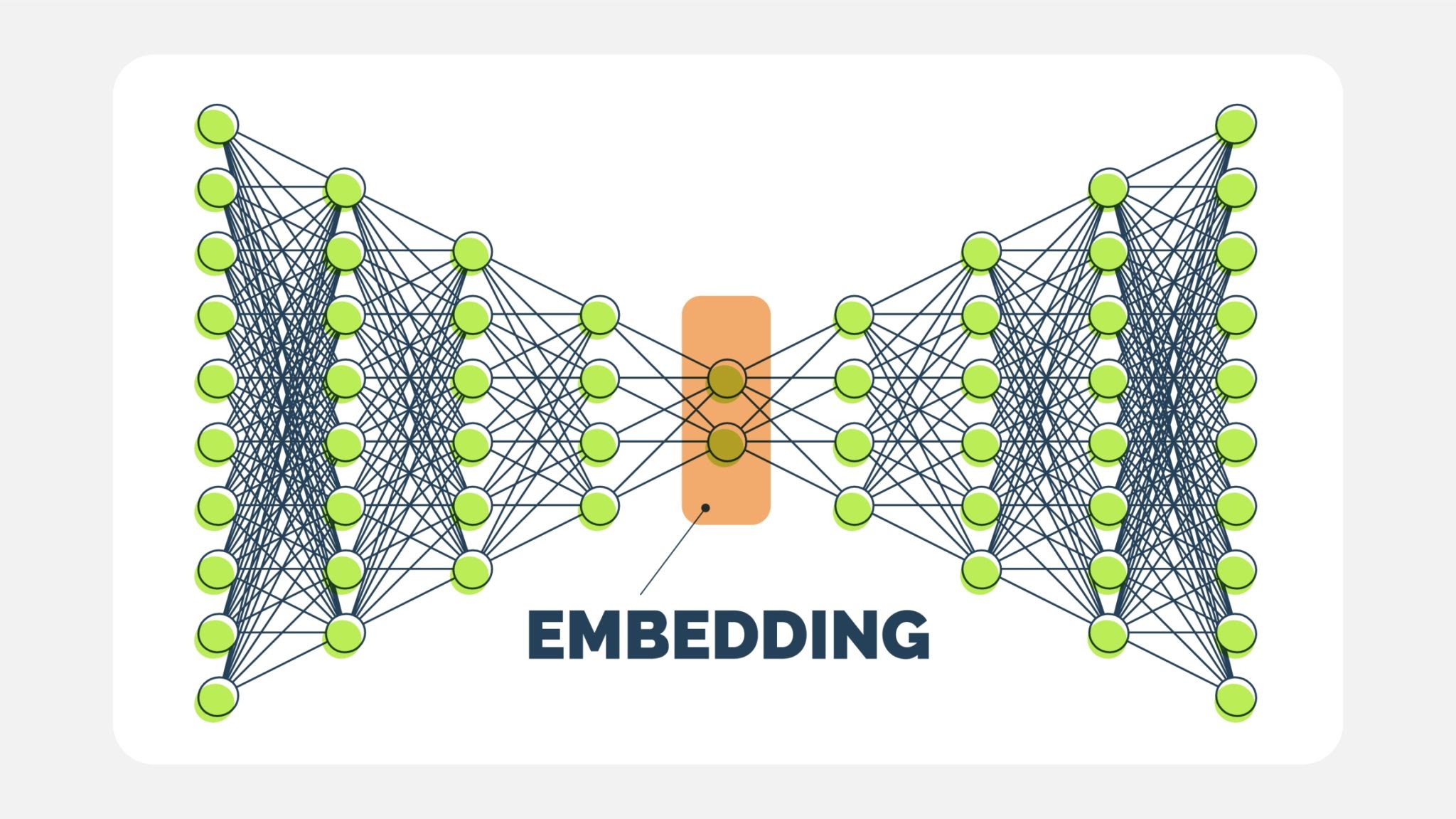
Autoencoder Model for Genotype Data Imputation

The Autoencoder model is designed to impute missing genotype data by encoding input data into a lower-dimensional latent representation and reconstructing the original input. This process helps capture complex patterns in the data and effectively handles missing values.

Model Overview

An autoencoder consists of two main components:

1. Encoder: Maps the high-dimensional input data to a lower-dimensional latent space.

2. Decoder: Reconstructs the input data from the latent representation.

The model aims to minimize the reconstruction loss between the original and reconstructed inputs.

Encoder Network

The encoder network transforms the input data through several hidden layers:

\[ \begin{align}\begin{aligned}\mathbf{H}_{1} = \sigma(\mathbf{W}_{1} \mathbf{X} + \mathbf{b}_{1})\\\mathbf{H}_{2} = \sigma(\mathbf{W}_{2} \mathbf{H}_{1} + \mathbf{b}_{2})\\\vdots\\\mathbf{Z} = \sigma(\mathbf{W}_{L} \mathbf{H}_{L-1} + \mathbf{b}_{L})\end{aligned}\end{align} \]

where:

• \(\mathbf{X} \in \mathbb{R}^{n \times d}\) is the input data.

• \(\mathbf{H}_{i}\) is the hidden representation at layer \(i\).

• \(\mathbf{W}_{i}\) and \(\mathbf{b}_{i}\) are the weights and biases of the encoder.

• \(\sigma\) is the activation function.

• \(\mathbf{Z}\) is the latent representation of dimension \(k\).

Decoder Network

The decoder reconstructs the original input data from the latent representation:

\[ \begin{align}\begin{aligned}\mathbf{H}_{i} = \sigma(\mathbf{W}_{i} \mathbf{H}_{i-1} + \mathbf{b}_{i})\\\mathbf{\hat{X}} = \sigma(\mathbf{W}_{\text{out}} \mathbf{H}_{L} + \mathbf{b}_{\text{out}})\end{aligned}\end{align} \]

where:

• \(\mathbf{\hat{X}}\) is the reconstructed input.

Loss Function

The model uses a masked focal loss to handle missing values and focus on difficult-to-predict data points. The masked focal loss is defined as:

\[\mathcal{L}_{\text{focal}}(p_t) = - \alpha_t (1 - p_t)^{\gamma} \log(p_t)\]

The overall loss is computed only over valid (unmasked) entries:

\[\mathcal{L} = \frac{1}{|M|} \sum_{(i,j) \in M} \mathcal{L}_{\text{focal}}(p_t)\]

Training Procedure

The autoencoder is trained using backpropagation with the AdamW optimizer and a warmup-to-cosine learning rate schedule. The key steps in training are:

1. Forward pass: Compute the output of the model.

2. Compute loss: Calculate the masked focal loss between the original and reconstructed inputs.

3. Backpropagation: Compute the gradients of the loss.

4. Update parameters: Update the weights and biases of the encoder and decoder.

PG-SUI can anneal focal-loss gamma from 0 to the configured value when train.gamma_schedule is enabled.

Variational Autoencoder (VAE) Model for Genotype Data Imputation

The Variational Autoencoder (VAE) model is designed to impute missing genotype data using a probabilistic approach. The model learns a distribution over the latent space and samples from this distribution to reconstruct the input data.

Model Overview

A VAE consists of three key components:

1. Encoder: Maps the input data to a distribution in the latent space.

2. Latent Space Sampling: Samples latent variables from the distribution defined by the encoder.

3. Decoder: Reconstructs the input data from the sampled latent variables.

Encoder Network

The encoder maps the input \(\mathbf{X}\) to the parameters of a Gaussian distribution over the latent space:

\[ \begin{align}\begin{aligned}\mu = f_{\mu}(\mathbf{X})\\\log \sigma^{2} = f_{\sigma}(\mathbf{X})\end{aligned}\end{align} \]

where:

• \(\mu\) is the mean of the distribution.

• \(\sigma^{2}\) is the variance.

• \(f_{\mu}\) and \(f_{\sigma}\) are neural networks representing the encoder.

Latent Space Sampling

The model samples a latent variable \(\mathbf{z}\) using the reparameterization trick:

\[\mathbf{z} = \mu + \epsilon \cdot \sigma, \quad \epsilon \sim \mathcal{N}(0, \mathbf{I})\]

This allows the model to backpropagate through the sampling step during training.

Decoder Network

The decoder reconstructs the input data from the sampled latent variables:

\[\mathbf{\hat{X}} = f_{\text{dec}}(\mathbf{z})\]

where \(f_{\text{dec}}\) is a neural network representing the decoder.

Loss Function

The VAE loss consists of two components:

1. Reconstruction Loss: Measures the difference between the original and reconstructed inputs using a masked focal loss:

   \[\mathcal{L}_{\text{recon}} = \frac{1}{|M|} \sum_{(i,j) \in M} \alpha_t (1 - p_t)^{\gamma} \log(p_t)\]

2. KL Divergence: Regularizes the learned latent distribution to be close to the prior distribution (a standard normal distribution):

   \[\mathcal{L}_{\text{KL}} = D_{\text{KL}}(q(\mathbf{z} | \mathbf{X}) \| p(\mathbf{z}))\]

The total loss is given by:

\[\mathcal{L} = \mathcal{L}_{\text{recon}} + \beta \mathcal{L}_{\text{KL}}\]

where \(\beta\) is a weighting factor that balances the reconstruction and KL divergence losses.

PG-SUI optionally anneals both \(\beta\) and focal-loss gamma during training, and scales the reconstruction term by the average number of masked loci per sample to keep the KL term from dominating on large matrices.

Non-linear PCA (NLPCA) Model for Genotype Data Imputation

Non-linear PCA (NLPCA) in PG-SUI is a decoder-only neural model. Instead of learning an encoder, it directly optimizes a latent embedding for each sample and learns a decoder that maps the embedding to genotype logits.

Model Overview

Let \(X \in \mathbb{R}^{N \times L}\) be the genotype matrix (0/1/2 with missing entries set to -1). Each sample \(i\) has a latent vector \(v_i \in \mathbb{R}^K\), and a shared decoder \(f_W\) predicts per-locus class logits:

\[\hat{X}_i = f_W(v_i)\]

Loss Function

The NLPCA objective uses a masked focal cross-entropy loss evaluated only on observed entries, with optional class weights and L1 regularization:

\[\mathcal{L} = \frac{1}{|M|} \sum_{(i,j) \in M} w_{y_{ij}} (1 - p_{ij})^{\gamma} \log(p_{ij}) + \lambda \lVert W \rVert_1\]

where \(M\) indexes non-missing entries, \(p_{ij}\) is the probability assigned to the true genotype class, and \(\gamma\) is the focal-loss parameter.

Training Procedure

1. PCA initialization: latent vectors are initialized with PCA on observed training data.

2. Working-matrix initialization: originally missing entries are filled with per-locus mode values; simulated-missing entries remain masked.

3. Joint optimization: embeddings and decoder weights are optimized together via backpropagation.

4. Input refinement: after selected epochs, originally missing entries are replaced with current reconstructions while simulated-missing entries remain masked.

5. Projection evaluation: validation/inference refines latent vectors with the decoder fixed, improving reconstruction before scoring.

Unsupervised Backpropagation (UBP) Model for Genotype Data Imputation

Unsupervised Backpropagation (UBP) also uses a decoder-only model with per-sample latent embeddings. PG-SUI follows a phased optimization schedule based on Gashler et al. (2014), combining PCA initialization with joint refinement.

Model Overview

Like NLPCA, UBP predicts genotypes via a decoder \(f_W\):

\[\hat{X}_i = f_W(v_i)\]

The loss uses the same masked focal cross-entropy with optional L1 regularizer on decoder weights:

\[\mathcal{L} = \frac{1}{|M|} \sum_{(i,j) \in M} w_{y_{ij}} (1 - p_{ij})^{\gamma} \log(p_{ij}) + \lambda \lVert W \rVert_1\]

Training Phases

1. Initialization: PCA provides a warm-start for the latent embeddings.

2. Decoder refinement: freeze embeddings and optimize decoder weights.

3. Joint refinement: optimize embeddings and decoder weights together, allowing the latent manifold to become non-linear.

During evaluation and inference, PG-SUI refines embeddings via projection with the decoder frozen, then scores or imputes genotypes.

IterativeImputer and the MICE Algorithm

IterativeImputer in scikit-learn is a general-purpose multiple imputation strategy that iteratively models each SNP column based on the most correlated loci.

Multivariate Imputation by Chained Equations (MICE)

MICE performs sequential regression-based imputation, where each missing value is predicted iteratively based on other features.

Let:

• \(X = (X_1, X_2, ..., X_p)\) be the SNP dataset with missing values.

• \(X_{-j}\) be all columns except the \(jth\) one.

For each column \(X_j\):

1. Initialize missing values using a simple strategy (e.g., mean imputation).

2. Train a regression model \(f_j\) predicting \(X_j\) using \(X_{-j}\):

\[X_j = f_j(X_{-j}) + \epsilon\]

where \(f_j\) is a regression model (e.g., Random Forest, HistGradientBoosting).

3. Predict missing values in \(X_j\) using \(f_j\).

4. Repeat for all columns and cycle multiple times (controlled by max_iter).

The process stops when convergence is reached (i.e., imputed values stabilize across iterations).

Further Reading

For additional details, refer to the scikit-learn documentation: https://scikit-learn.org/stable/modules/impute.html#iterative-imputer

Conclusion

PG-SUI provides a range of deep learning, machine learning, and statistical methods for SNP imputation. ImputeAutoencoder, ImputeVAE, ImputeNLPCA, and ImputeUBP cover deep learning approaches, and the IterativeImputer framework enables regression-based imputation.

For more details, see the PG-SUI API documentation.